Flank-context spectra of RIP-like sites (Python API)

Not every RIP substrate is converted. deRIP2 can ask whether a local sequence context protects a substrate from RIP by classifying every RIP-like dinucleotide by the single base 1 bp upstream and 1 bp downstream — a 4 bp motif [up][centre][down] with the two centre bases fixed and the flanks varying, giving 16 channels. Two site states are counted:

• Substrate — surviving CpA (forward) / TpG (reverse), counted anywhere in each sequence.
• Product — realised TpA in a RIP-informative column.

Reverse-strand motifs are reverse-complemented onto the CpA/TpA strand, so a substrate GCAG and its product GTAG share one flank channel (the CA-state label GCAG).

The per-sequence HTML report renders this automatically (see Per-sequence Reporting). This page shows how to drive the same analysis from Python: extract the spectra, plot them, rank motifs by conversion, compare two spectra sets, and flag the individual motifs that differ — with a note on normalising for sample size.

Extracting the spectra

Run RIP detection, then compute the flank spectra. The result is a FlankSpectraResult with one sample column per input sequence.

from derip2.derip import DeRIP

d = DeRIP("tests/data/sahana.fasta.gz")
d.calculate_rip()
result = d.calculate_flank_spectra()      # cached on d.flank_spectra_result

result.sample_names          # one label per aligned sequence
result.channels_substrate    # 16 CA-state motifs: ['ACAA', 'ACAC', ..., 'TCAT']
result.channels_product      # the equivalent TA-state motifs: ['ATAA', ...]

Each state/strand is a (16, n_sequences) count matrix. Pull them with .matrix(state, strand), or pool every sequence into a single alignment-wide spectrum with .pooled():

import numpy as np

# Per-sequence, combined strands:
sub_by_seq = result.matrix("substrate", "combined")   # (16, n_sequences)
prod_by_seq = result.matrix("product", "combined")

# Alignment-wide (pooled) 16-vectors:
pooled = result.pooled()                               # dict of (16,) vectors
substrate = pooled["sub_fwd"] + pooled["sub_rev"]      # combined substrate
product = pooled["prod_fwd"] + pooled["prod_rev"]      # combined product
motifs = result.channels_substrate

state is "substrate" or "product"; strand is "combined", "forward" or "reverse". Substrate counts use the raw CpA/TpG masks (every surviving substrate), while product counts are gated to RIP-informative columns — this asymmetry is deliberate. Sites at an alignment edge that lack a resolvable 4 bp context are dropped and tallied in result.n_skipped_flank.

To compute directly from a ColumnClassification (e.g. outside a DeRIP object), call the underlying function:

from derip2.stats.flank_spectra import compute_flank_spectra

ids = [record.id for record in d.alignment]
result = compute_flank_spectra(d.column_classes, sample_names=ids)

Plotting

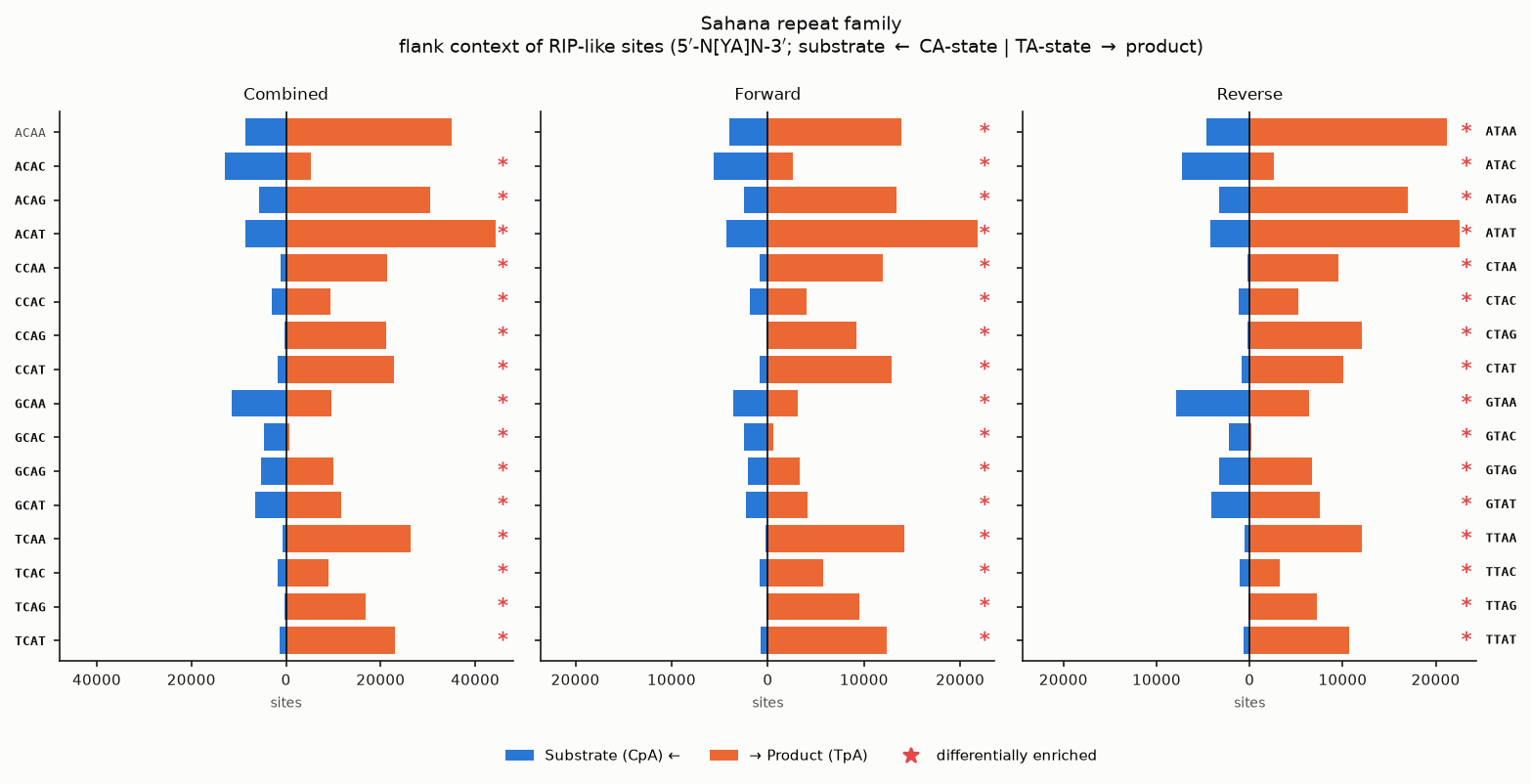
DeRIP.plot_flank_spectra() draws the pooled bihistograms (substrate left, product right; CA-state motif on the left axis, TA-state on the right; motifs that differ significantly between states marked *):

fig = d.plot_flank_spectra(title="Sahana repeat family")
fig.savefig("sahana_flank.png", dpi=150, bbox_inches="tight")

Count-normalised proportions

By default the bars are raw counts. There are usually far more substrate sites than product sites (substrate is counted everywhere, product only in RIP columns), so the raw bihistogram is dominated by that overall imbalance. Pass percentage=True to plot count-normalised proportions instead: each state is rescaled to sum to 100 % across the 16 motifs, so the substrate and product shapes are compared on equal footing and you can see which contexts are over- or under-represented in one state relative to the other.

# Each state normalised to 100 % of its own sites (x-axis: "% of state"):
fig = d.plot_flank_spectra(title="Sahana repeat family", percentage=True)
fig.savefig("sahana_flank_proportions.png", dpi=150, bbox_inches="tight")

For finer control use the plotting functions directly. strands selects which panels to draw (the report overview uses ("combined",)); sample picks one sequence; percentage works here too:

from derip2.plotting.flank_spectra import (
    plot_flank_bihistograms,          # one sequence
    plot_flank_bihistograms_pooled,   # all sequences pooled
)

# Just the combined panel, pooled across the alignment, as proportions:
plot_flank_bihistograms_pooled(
    result, strands=("combined",), percentage=True, outfile="combined.png"
)

# All three strand panels for the first sequence (raw counts):
plot_flank_bihistograms(result, sample=0, outfile="seq0_flank.png")

Flank-interaction conversion heatmap

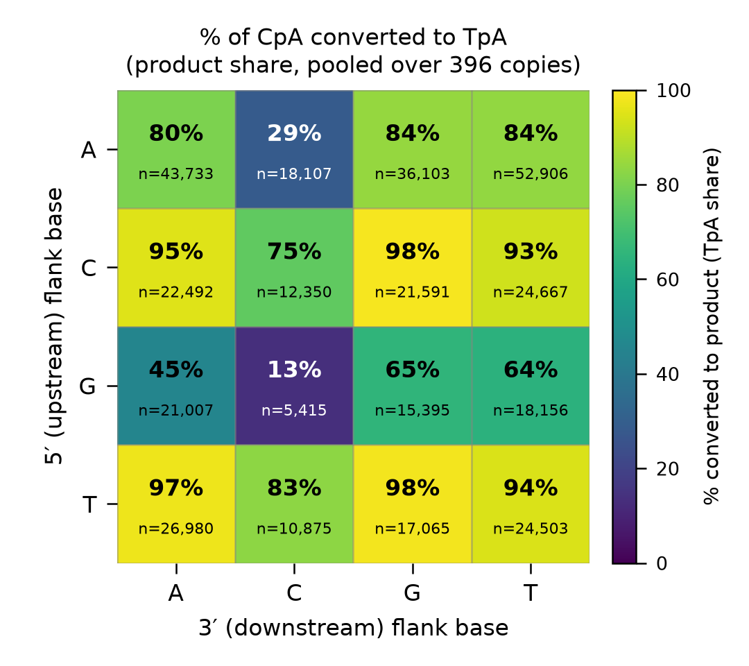
The bihistogram treats the two flanks together as one 16-way channel. To see how the 5′ and 3′ bases interact, plot the product share — product / (substrate + product), the fraction of each target CpA converted to TpA — as a 2-D heatmap with the 5′ (upstream) base on the rows and the 3′ (downstream) base on the columns. DeRIP.plot_flank_conversion_heatmap() recomputes the spectra at the requested flank_length and draws the grid; at 1 bp (4×4) each cell is annotated with its percentage and site count n, and colour-only for wider flanks.

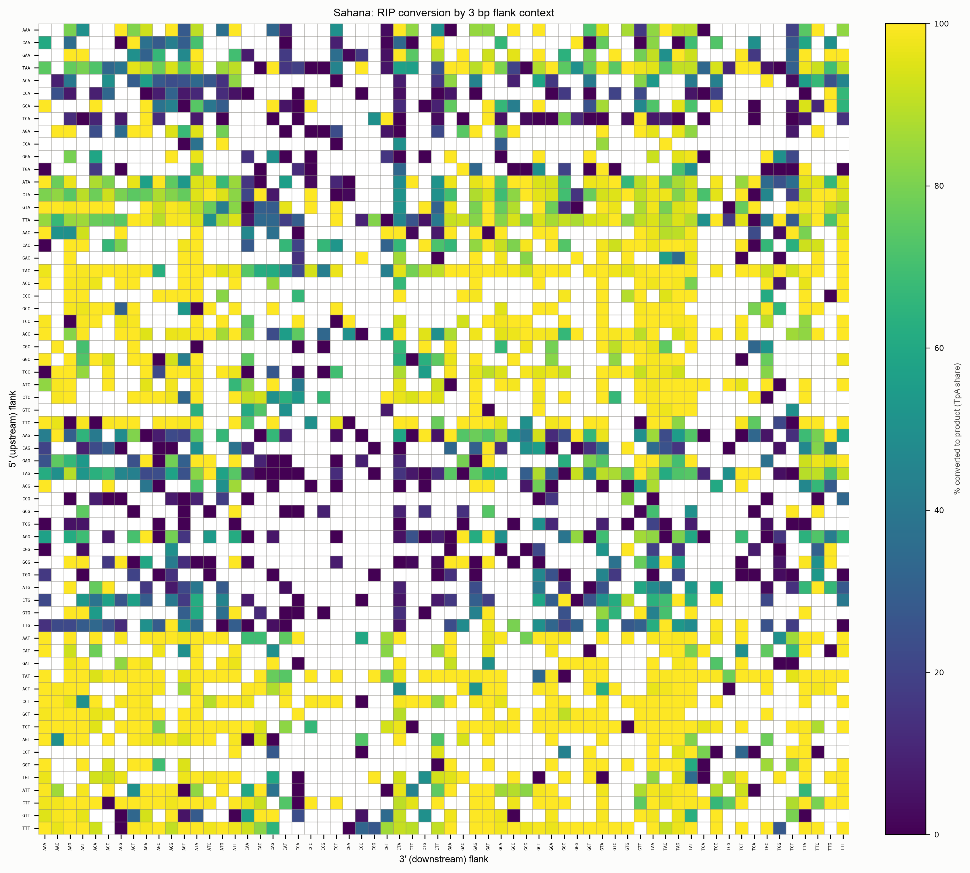
Colour defaults to viridis: dark purple where the motif has kept its substrate, through teal and green, to bright yellow where it has been fully converted. Note this is a magnitude scale — unlike the bihistograms, where blue and orange name the substrate and product states, hue here only tracks how far the conversion has gone. Motifs seen zero times are left white, reading as a hole in the grid rather than a low conversion rate (on the 3 bp grid roughly half the cells are blank).

Pass cmap to restyle the scale. It accepts any registered matplotlib colormap name (append _r to reverse it), a Colormap object, or a list of colours to interpolate between, low value first:

d.plot_flank_conversion_heatmap(output_file="heat_magma.png", cmap="magma_r")
d.plot_flank_conversion_heatmap(output_file="heat_custom.png",
                                cmap=["#ffffff", "#2a78d6", "#0b2b52"])

for w in (1, 2, 3):
    d.plot_flank_conversion_heatmap(
        output_file=f"sahana_flank_heatmap_{w}bp.png",
        flank_length=w,
        title=f"Sahana: RIP conversion by {w} bp flank context",
    )

At 1 bp the interaction is stark: a 3′ cytosine is protective almost regardless of the 5′ base (the C column stays darkest — GCAC only 13 % converted), while every other 3′ base exceeds ~60 %.

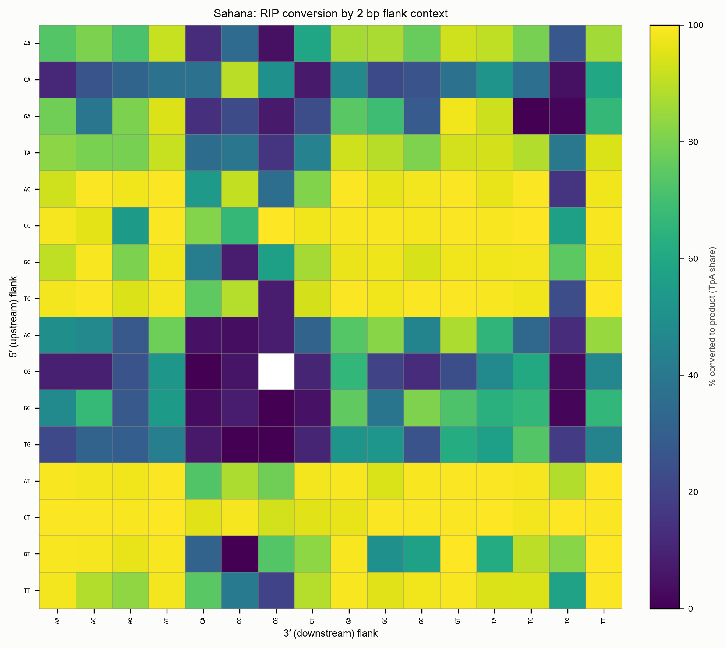
Widening the flank to 2 bp (16×16, 5′/3′ dinucleotides) and 3 bp (64×64, 5′/3′ trinucleotides) resolves the context further. The nearest-base bands persist — the signal is carried by the two bases immediately flanking the target — but the counts per motif thin quickly (only about half of the 4,096 three-flank motifs occur in the family, so many 3 bp cells are blank). Read a low- or high-conversion cell together with its n: extreme rates on a handful of sites are not reliable.

For finer control (single sequence, flank ordering, no title) call the plotting function directly on a pre-computed result:

from derip2.plotting.flank_spectra import plot_flank_conversion_heatmap

result2 = d.calculate_flank_spectra(flank_length=2)
plot_flank_conversion_heatmap(
    result2, sample=None, flank_sort="proximal", outfile="heatmap_2bp.png"
)

To pool this analysis across many independent alignments — different families or species — with sample-size-weighted rates and confidence intervals, see Combined spectra across many alignments.

Ranking motifs by RIP conversion

The biologically interesting quantity is the product share of each flank context — product / (substrate + product) — i.e. how readily that context is converted to RIP product. Rank the motifs by it:

total = substrate + product
with np.errstate(invalid="ignore"):
    pct_converted = np.where(total > 0, 100.0 * product / total, np.nan)

order = np.argsort(-np.nan_to_num(pct_converted))     # most-converted first
for i in order[:5]:
    print(f"{motifs[i]}  {pct_converted[i]:5.1f}%  (n={int(total[i])})")

CCAG   98.5%  (n=21591)
TCAG   98.4%  (n=17065)
TCAA   97.4%  (n=26980)
...

Always read the percentage next to the total n: a context with only a handful of sites can show an extreme conversion rate by chance. This is exactly the Motif / Substrate / Product / Total / % RIP table rendered (and sortable) in the HTML report.

Comparing two sets of spectra

To ask whether two spectra differ — two families, two clades, or substrate vs product within one alignment — use derip2.stats.spectra_compare.compare_spectra, which returns a scale-free cosine similarity (shape), the χ² homogeneity test (significance) and Cramér's V (effect size):

from derip2.stats.spectra_compare import compare_spectra

cmp = compare_spectra(substrate, product, channels=motifs)
cmp["cosine_similarity"]   # 1.0 = identical flank preference
cmp["cramers_v"]           # effect size in [0, 1]
cmp["pvalue"]              # chi-squared homogeneity p-value
cmp["top_channels"]        # the most-differentiating motifs

For the five built-in substrate-vs-product / strand comparisons in one call, use compare_flank_spectra (per sequence) or compare_flank_spectra_pooled (alignment-wide):

from derip2.stats.flank_spectra import compare_flank_spectra_pooled

comparisons = compare_flank_spectra_pooled(result)
comparisons["sub_vs_prod_combined"]["cosine_similarity"]
comparisons["fwd_vs_rev_product"]["cramers_v"]

Each comparison carries a chi2_reliable flag (both spectra have ≥ min_sites sites); the report only shows a p-value when it is set.

Identifying individually-different motifs

differential_channels flags which motifs drive a substrate-vs-product difference. For each of the 16 contexts it forms one row of a 16×2 table and tests that cell's adjusted standardised (Haberman) residual against the standard normal — a motif is flagged when |z| ≥ z(α) (two-sided), provided both states have at least min_sites sites, with no multiple-testing correction:

from derip2.stats.flank_spectra import differential_channels

flagged = differential_channels(substrate, product, min_sites=20, alpha=0.05)
[motifs[i] for i in np.nonzero(flagged)[0]]     # significantly enriched motifs

These are the motifs marked * on the bihistograms. The same function works on any two 16-vectors, e.g. the product spectra of two different families.

Normalising for sample size

Counts scale with alignment size and RIP load, so be deliberate when comparing:

• Cosine similarity is already scale-free. It compares the shape of two spectra, so compare_spectra(a, b) gives the same value whether a/b are raw counts or proportions. Reach for it first when the two spectra have very different totals.

# identical cosine, whether counts or proportions:
sp, pp = substrate / substrate.sum(), product / product.sum()
compare_spectra(sp, pp)["cosine_similarity"] == compare_spectra(substrate, product)["cosine_similarity"]

• The χ² p-value is powered by n. With large pooled counts almost every context becomes "significant" (on the full Sahana family nearly all 16 motifs flag), so lead with the effect sizes — cosine and Cramér's V — and treat the p-value as a yes/no on whether there is any difference, not how much.

• To compare composition across samples of different sizes, normalise each spectrum to proportions (divide by its own total, or use the percentage=True option on the plot functions) before eyeballing them. Keep the raw counts for the tests, which need integer frequencies.

• Per-sequence spectra are small. The min_sites gate (default 20) stops differential_channels and the report's per-motif marks from over-interpreting a sequence with only a few RIP-like sites; raise it for noisier data.

Writing the tables

The tidy count matrix and comparison statistics can be written straight to TSV (these are also emitted next to the HTML report):

d.write_flank_spectra_matrix("rip_context_spectra.tsv")        # sample x state x strand x channel
d.write_flank_spectra_comparisons("rip_context_comparisons.tsv")

See also

• Per-sequence Reporting — the HTML section that renders these spectra, the sortable per-motif table, and the comparisons.
• Mutation spectra — the SBS-96/192 substitution spectra (a different context model for the same substitutions).