Combined spectra across many alignments (Python API)

A single alignment tells you how RIP shaped one transposon family. To ask what RIP does in general — across many families, or across a panel of species — you need to combine the spectra of many independent alignments into one signature. This page shows how to drive deRIP2's per-alignment spectra over a corpus of MSAs and pool them into three combined views:

the SBS-96 mutation spectrum,
the 16-channel flank-context bihistogram of RIP substrate/product sites,
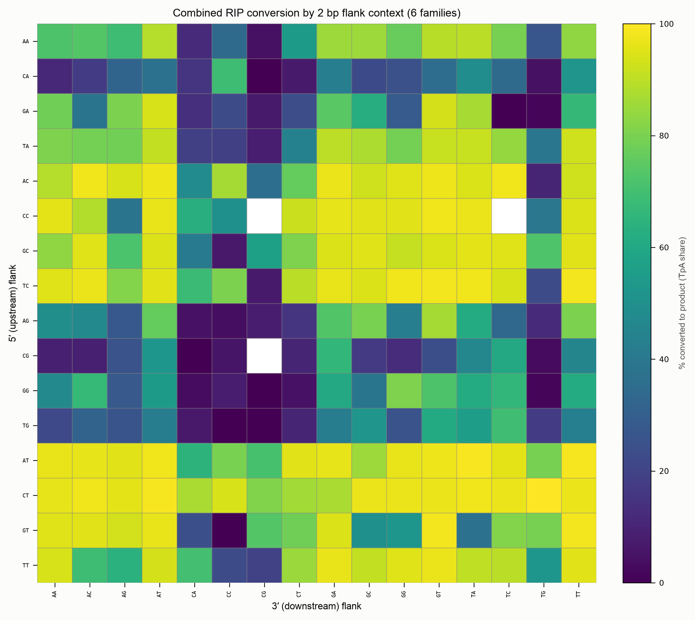
the configurable-width flank RIP-conversion heatmap (1/2/3 bp).

The one genuinely tricky part is combining conversion rates, so we deal with it head-on: pool counts, don't average percentages.

Reproducible demo

Every snippet below runs against the bundled tests/data/sahana.fasta.gz, which we split into groups to simulate independent families. For real work, replace the loop over groups with a loop over your own per-family FASTA files — the aggregation code is identical.

Extracting one alignment at a time

For each alignment, run RIP detection once, then pull the pooled flank spectra (at each flank width you care about) and the pooled SBS-96 spectrum. We keep only the compact count vectors so many families fit comfortably in memory.

import gzip
import numpy as np
from Bio import SeqIO
from Bio.Align import MultipleSeqAlignment
from derip2.derip import DeRIP

FLANK_WIDTHS = (1, 2, 3)

def extract_family(aln):
    """Return pooled flank substrate/product counts and the SBS-96 vector."""
    d = DeRIP(aln)
    d.calculate_rip()
    flank = {}
    for w in FLANK_WIDTHS:
        pooled = d.calculate_flank_spectra(flank_length=w).pooled()
        flank[w] = {
            "substrate": pooled["sub_fwd"] + pooled["sub_rev"],   # (4**2w,)
            "product":   pooled["prod_fwd"] + pooled["prod_rev"],
        }
    sbs = d.calculate_spectra(partition_by="none").sbs96[:, 0]     # (96,)
    return {"n_seqs": len(aln), "flank": flank, "sbs96": sbs}

Now build the corpus. In the demo we split Sahana into six contiguous groups; for real data you would iterate over glob.glob("family_msas/*.fasta") and read each file instead.

import math

records = list(SeqIO.parse(gzip.open("tests/data/sahana.fasta.gz", "rt"), "fasta"))
size = math.ceil(len(records) / 6)
groups = [records[i:i + size] for i in range(0, len(records), size)]

per_family = [extract_family(MultipleSeqAlignment(g)) for g in groups if len(g) >= 2]
print(f"{len(per_family)} families, {sum(f['n_seqs'] for f in per_family)} sequences")

Pooling: why counts, not rates

The biologically interesting quantity is each flank motif's product share — product / (substrate + product), the fraction of that context converted to RIP product. The wrong way to combine it across families is to average the per-family percentages: families differ enormously in how many sites of each motif they carry, so a family with three sites of a rare motif would count as much as one with thirty thousand.

Instead, pool the counts. Summing substrate and product across families and then taking the ratio gives a binomial success rate whose precision scales with the pooled sample size — automatically sample-size-weighted:

def pool_flank(per_family, width):
    n = 4 ** (2 * width)
    substrate = np.zeros(n, dtype=np.int64)
    product = np.zeros(n, dtype=np.int64)
    for f in per_family:
        substrate += f["flank"][width]["substrate"].astype(np.int64)
        product += f["flank"][width]["product"].astype(np.int64)
    total = substrate + product
    with np.errstate(invalid="ignore", divide="ignore"):
        rate = np.where(total > 0, product / total, np.nan)     # pooled % conversion
    return substrate, product, total, rate

The error margin: a Wilson confidence interval

A pooled rate is only as trustworthy as its n. Attach a Wilson score 95 % confidence interval — it stays inside [0, 1] and behaves well at extreme rates and small counts, unlike the textbook normal interval, which is exactly the regime of rarely-seen motifs. (This needs only math; no SciPy.)

import math

def wilson_ci(success, n, alpha=0.05):
    if n <= 0:
        return (float("nan"), float("nan"))
    z = 1.959963984540054                       # normal quantile for alpha=0.05
    p = success / n
    denom = 1 + z * z / n
    centre = (p + z * z / (2 * n)) / denom
    half = (z / denom) * math.sqrt(p * (1 - p) / n + z * z / (4 * n * n))
    return (max(0.0, centre - half), min(1.0, centre + half))

sub, prod, total, rate = pool_flank(per_family, 1)
for i in np.argsort(-np.nan_to_num(rate))[:5]:
    lo, hi = wilson_ci(int(prod[i]), int(total[i]))
    print(f"motif {i:2d}  {rate[i]*100:5.1f}%  [{lo*100:4.1f}, {hi*100:4.1f}]  n={total[i]:,}")

Between-family variability

Pooling answers "what is the conversion rate overall", but hides whether families agree. Keep that signal by also computing each family's own rate (gated to families with enough sites) and reporting the mean ± SD across families. A high SD flags a motif whose conversion is family-dependent rather than universal.

def family_dispersion(per_family, width, min_sites=20):
    rates = []
    for f in per_family:
        s = f["flank"][width]["substrate"].astype(float)
        p = f["flank"][width]["product"].astype(float)
        tot = s + p
        with np.errstate(invalid="ignore", divide="ignore"):
            rates.append(np.where(tot >= min_sites, p / tot, np.nan))
    rates = np.vstack(rates)
    return np.nanmean(rates, axis=0), np.nanstd(rates, axis=0)   # mean, SD per motif

Read the pooled rate and the family SD together

A motif can show a confident pooled rate (tight Wilson CI, because n is large) yet still vary widely between families (large SD). The CI is sampling uncertainty; the SD is biological heterogeneity — they answer different questions.

Plotting the combined views

deRIP2's plotters take a result object, not raw arrays. Rather than reimplement them, synthesise a single-column result from the pooled counts and hand it straight to the stock plotters. Both result types are dataclasses, so this is a one-liner per view.

Combined flank heatmaps (1/2/3 bp)

Place the pooled substrate/product totals on a one-sample FlankSpectraResult and call the stock heatmap:

from derip2.stats.flank_spectra import FlankSpectraResult
from derip2.spectra.flank_channels import flank_channel_labels
from derip2.plotting.flank_spectra import plot_flank_conversion_heatmap

def combined_flank_result(per_family, width):
    sub, prod, _total, _rate = pool_flank(per_family, width)
    n = sub.shape[0]
    zero = np.zeros((n, 1))
    return FlankSpectraResult(
        sub_fwd=sub.astype(float)[:, None], sub_rev=zero.copy(),
        prod_fwd=prod.astype(float)[:, None], prod_rev=zero.copy(),
        sample_names=[f"combined ({len(per_family)} families)"],
        n_skipped_flank={}, flank_length=width,
        channels_substrate=list(flank_channel_labels("CA", width=width)),
        channels_product=list(flank_channel_labels("TA", width=width)),
    )

for w in (2, 3):
    plot_flank_conversion_heatmap(
        combined_flank_result(per_family, w), sample=None,
        outfile=f"combined_flank_heatmap_{w}bp.png",
        title=f"Combined RIP conversion by {w} bp flank context",
    )

Combined 2 bp flank heatmap

The stock heatmap annotates counts but not the confidence interval. For the 4×4 1 bp grid there is room to show the pooled percentage, its Wilson CI half-width and the pooled n in every cell — and to hatch cells whose between-family SD is high. The experiments/combined_spectra/fig_flank_heatmaps.py script draws exactly this; it produces:

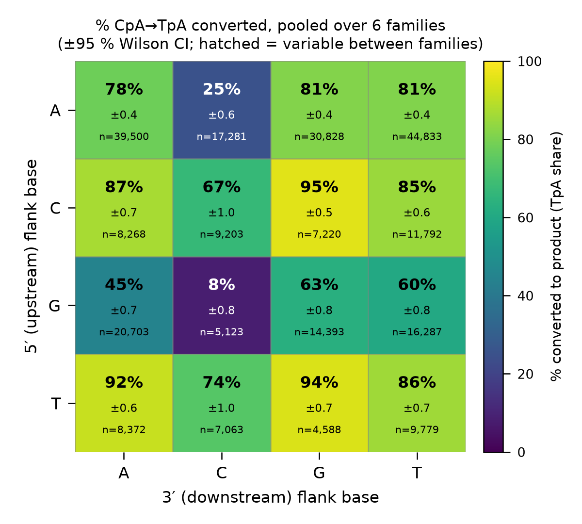
Combined 1 bp flank heatmap with CIs

The nearest-3′ C column is the darkest — a downstream cytosine protects the target CpA from RIP regardless of the 5′ base — reproducing the single-family result on a pooled, error-barred footing.

Combined SBS-96

Same idea with a one-sample SpectraResult; the SBS-96 plotter reads only the matrix and sample name, so the event-level fields can be left empty. Plot as percentage=True so families of different sizes compare on equal footing:

from derip2.stats.mutation_spectra import SpectraResult
from derip2.plotting.spectra import plot_sbs96

pooled96 = sum(f["sbs96"].astype(np.int64) for f in per_family)
empty_i, empty_s = np.zeros(0, dtype=int), np.zeros(0, dtype="S1")
combined_sbs = SpectraResult(
    sbs96=pooled96.astype(float)[:, None], sbs192=None,
    sample_names=[f"combined ({len(per_family)} families)"],
    event_rows=empty_i, event_cols=empty_i, event_ref=empty_s, event_alt=empty_s,
    event_five=empty_s, event_three=empty_s, event_sample=empty_i,
    homoplasy_counts=np.zeros((0, 4), dtype=int), ancestor_ref=empty_s,
    n_indel_or_ambiguous=0, n_unassignable_context=0,
)
plot_sbs96(combined_sbs, outfile="combined_sbs96.png", sample=0, percentage=True,
           title="Combined SBS-96 spectrum")

Combined SBS-96 spectrum

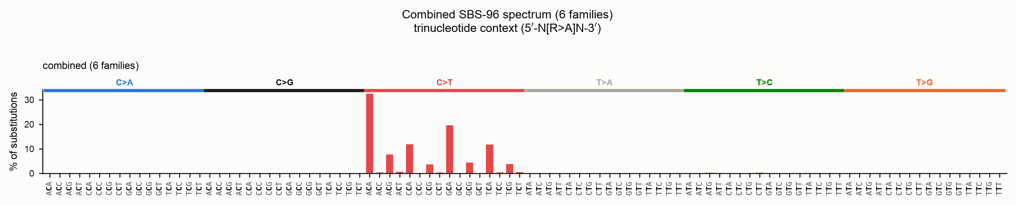
All the signal sits in the C>T block, concentrated in NCA contexts — the canonical RIP signature, now pooled across the whole corpus.

Combined bihistogram

Reuse the 1 bp combined_flank_result and draw the pooled bihistogram. Restrict it to the combined panel (the pooled counts have no meaningful per-strand split) and normalise each state to 100 % of its own sites:

from derip2.plotting.flank_spectra import plot_flank_bihistograms_pooled

plot_flank_bihistograms_pooled(
    combined_flank_result(per_family, 1), outfile="combined_flank_bihistogram.png",
    strands=("combined",), percentage=True, title="Combined flank-context spectra",
)

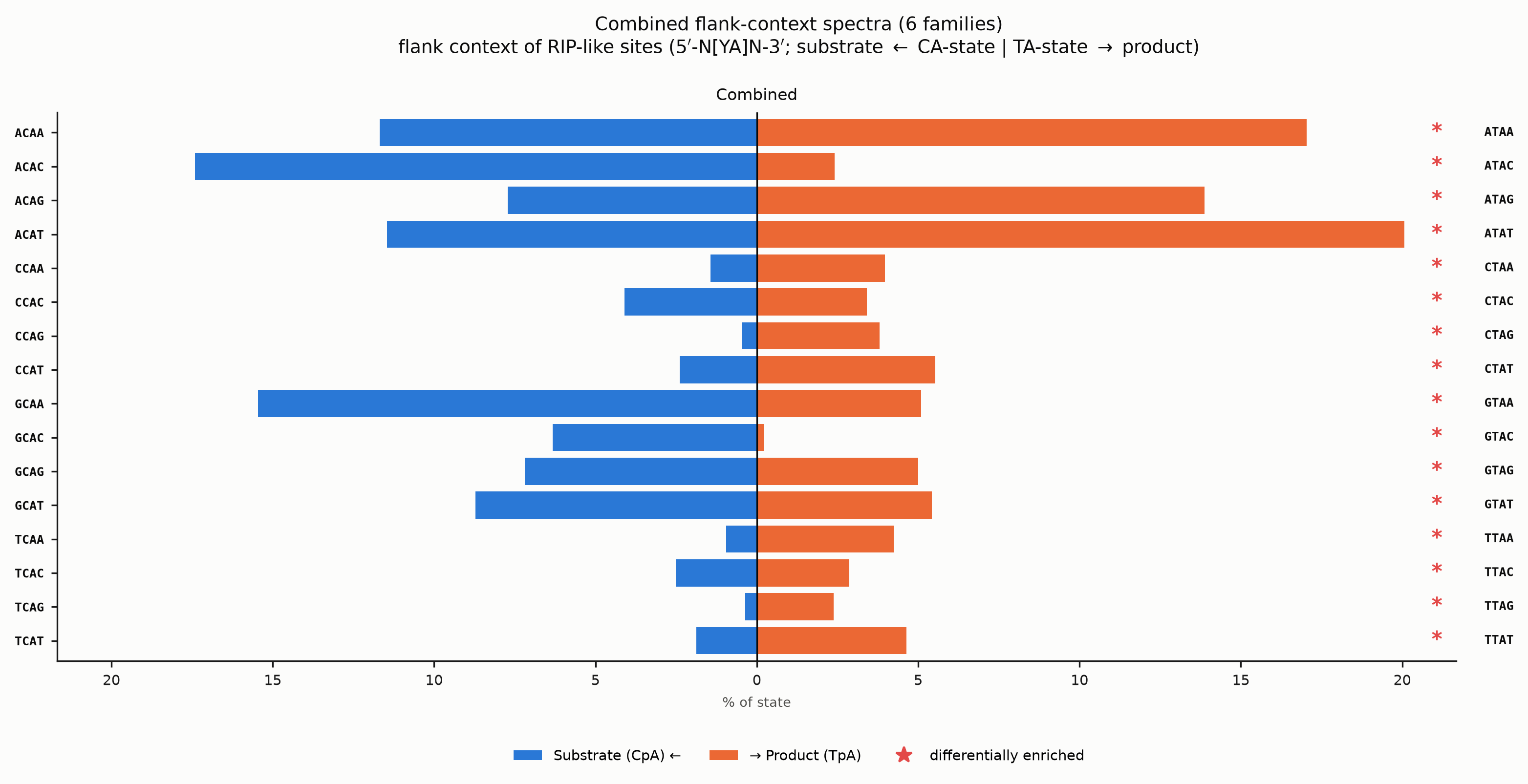
Combined flank-context bihistogram

Motifs whose substrate and product proportions differ significantly are marked * (via differential_channels).

Comparing the combined spectra of two panels

Once you have pooled spectra for two groups — say RIP-positive vs RIP-negative species — compare them with the scale-free tools from spectra_compare: cosine similarity for shape, χ² / Cramér's V for significance and effect size. Because cosine similarity is scale-free, it is unaffected by the two panels having very different total counts.

from derip2.stats.spectra_compare import compare_spectra

a = sum(f["sbs96"].astype(np.int64) for f in panel_a)
b = sum(f["sbs96"].astype(np.int64) for f in panel_b)
cmp = compare_spectra(a, b)
print(cmp["cosine_similarity"], cmp["cramers_v"], cmp["pvalue"])

Reproducing the manuscript figures

The experiments/combined_spectra/ scripts wrap everything above with per-family JSON caching and a --demo / --input-dir switch:

python experiments/combined_spectra/aggregate.py --input-dir family_msas -v
python experiments/combined_spectra/fig_flank_heatmaps.py           # 1/2/3 bp heatmaps
python experiments/combined_spectra/fig_sbs96_combined.py           # SBS-96
python experiments/combined_spectra/fig_flank_bihistogram_combined.py

Omit --input-dir for the reproducible Sahana demo used to render the figures on this page.