Why coverage dies at contig ends¶

Teloclip exists because of a sampling artefact: read coverage does not stay flat all the way to the end of a linear chromosome — it decays smoothly to zero over roughly one read length. Assemblers see thin, one-sided evidence in that window and stop early, which is why draft contigs so often end just short of the telomere. This page gives the statistical model behind that decay, so you can reason about how much overhang evidence to expect at a given depth and read-length profile.

If you have not already, read how overhangs are defined and telomere biology first — this page explains why the overhang reads those pages describe are always rarer than the interior depth suggests.

The model¶

Two random processes place a read on a molecule:

Fragmentation is uniform. Breakpoints fall anywhere along the molecule, so a fragment of length \(\ell\) can start at any position that lets it fit.
Size selection is a hard cutoff. Library preparation (or a read-length filter at mapping time) discards fragments shorter than some minimum \(L_{\min}\).

Consider a base at distance \(x\) from the terminus (\(x = 0\) is the outermost base). A fragment of length \(\ell\) covers it only if the fragment starts within the last \(x\) bases before it — there are \(\min(x + 1, \ell)\) such placements, against \(\ell\) placements for an interior base. A terminal base is simply a smaller target.

Averaging over the fragment-length distribution (truncated at \(L_{\min}\)) gives the expected coverage relative to the interior:

\[ c(x) \;=\; \frac{\mathbb{E}\left[\min(x + 1,\, \ell) \mid \ell \ge L_{\min}\right]} {\mathbb{E}\left[\ell \mid \ell \ge L_{\min}\right]} \]

Note the denominator: size selection also changes the interior mean fragment length, so both numerator and denominator use the truncated distribution. Absolute expected coverage is \(D \cdot c(x)\), where \(D\) is the interior depth after size selection.

What \(c(x)\) is normalised to

\(c(x)\) is coverage relative to the interior depth of the selected library — the reads that survive the cutoff. Because the survivors, however few, still fragment uniformly along the molecule, they tile the interior evenly and \(c(x) \to 1\) in the interior for any cutoff. What a harsh cutoff really costs is yield: at equal sequencing effort, only a fraction \(S(L_{\min}) \cdot \mathbb{E}[\ell \mid \ell \ge L_{\min}] / \mathbb{E}[\ell]\) of sequenced bases survive, so the absolute depth \(D\) drops everywhere. Panel b below adds that yield factor back by normalising to the unselected library's interior depth.

The model assumes the molecule is far longer than any fragment (semi-infinite): on a real chromosome the same decay is simply mirrored at the other terminus.

Fixed fragment length¶

If every fragment has length \(L\), the curve is a straight ramp:

\[ c(x) = \frac{\min(x + 1,\, L)}{L} \]

Coverage rises linearly from \(1/L\) at the outermost base and reaches the interior depth exactly one fragment length in.

Lognormal fragment lengths¶

Real long-read length profiles are well described by a lognormal. With \(\ell \sim \mathrm{Lognormal}(\mu, \sigma)\) (parameterised by the real-space mean \(m\) and standard deviation \(s\)), the partial expectation has a closed form in the normal CDF \(\Phi\):

\[ \mathbb{E}\left[\min(a, \ell)\right] = m\,\Phi\!\left(\frac{\ln a - \mu - \sigma^2}{\sigma}\right) + a\left(1 - \Phi\!\left(\frac{\ln a - \mu}{\sigma}\right)\right) \]

so \(c(x)\) is cheap to evaluate everywhere — no simulation needed. The decay is no longer linear: the long tail of the distribution reaches deeper into the contig, while short fragments (if they survive selection) soften the curve near the terminus.

What the curves look like¶

The figures below use a PacBio HiFi-like library: lognormal fragment lengths with mean 15 Kbp and sd 3 Kbp, and a strict lower-bound size-selection cutoff of 10 Kbp (every fragment shorter than the cutoff is discarded).

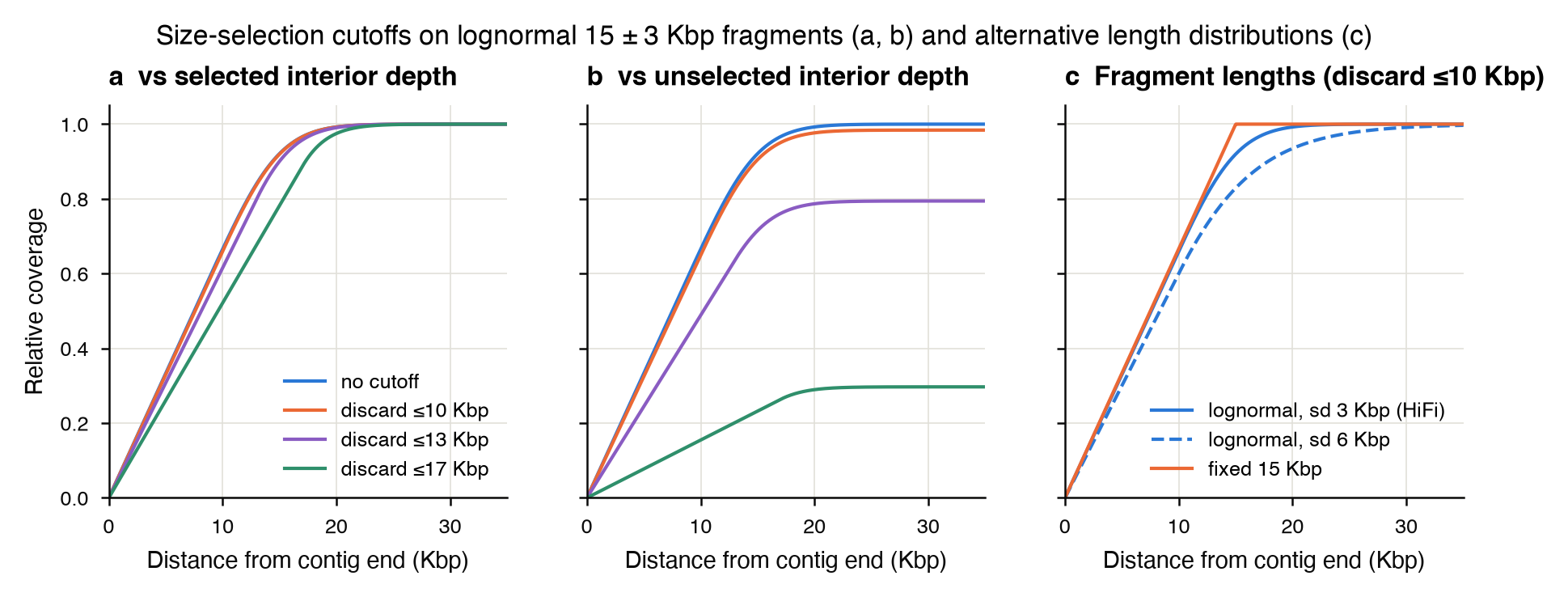
Four things to take away:

The decay region is about one (truncated) mean fragment length deep. With the 15 ± 3 Kbp HiFi profile, coverage within 5 Kbp of the terminus is only about a third of the interior depth, and interior depth is not reached until ~20 Kbp in.
Below the cutoff distance the curve is an exact straight line. Every surviving fragment is at least 10 Kbp, so for \(x < L_{\min}\) the number of placements that cover \(x\) grows linearly with \(x\) regardless of the length distribution — the distribution only shapes the shoulder beyond the cutoff.
Panel a shows shape; panel b shows shape plus yield. In panel a even the ≤17 Kbp curve reaches 1 in the interior, which can look wrong — the 15 ± 3 Kbp library has almost no fragments that long. It is correct because \(c(x)\) is normalised to the selected library's own interior depth (see the note above). Panel b renormalises to the unselected library: at equal sequencing effort the 10, 13 and 17 Kbp cutoffs retain ~98%, ~79% and ~30% of sequenced bases, which is where those interior plateaus land.
Cutoffs bite when they reach the typical length. The 10 Kbp HiFi cutoff discards only ~3% of fragments, so its curves sit almost on the no-cutoff curves in both panels; cutoffs approaching the mean (13 Kbp discards ~27% of fragments, 17 Kbp ~77%) deepen the depleted region and collapse yield.

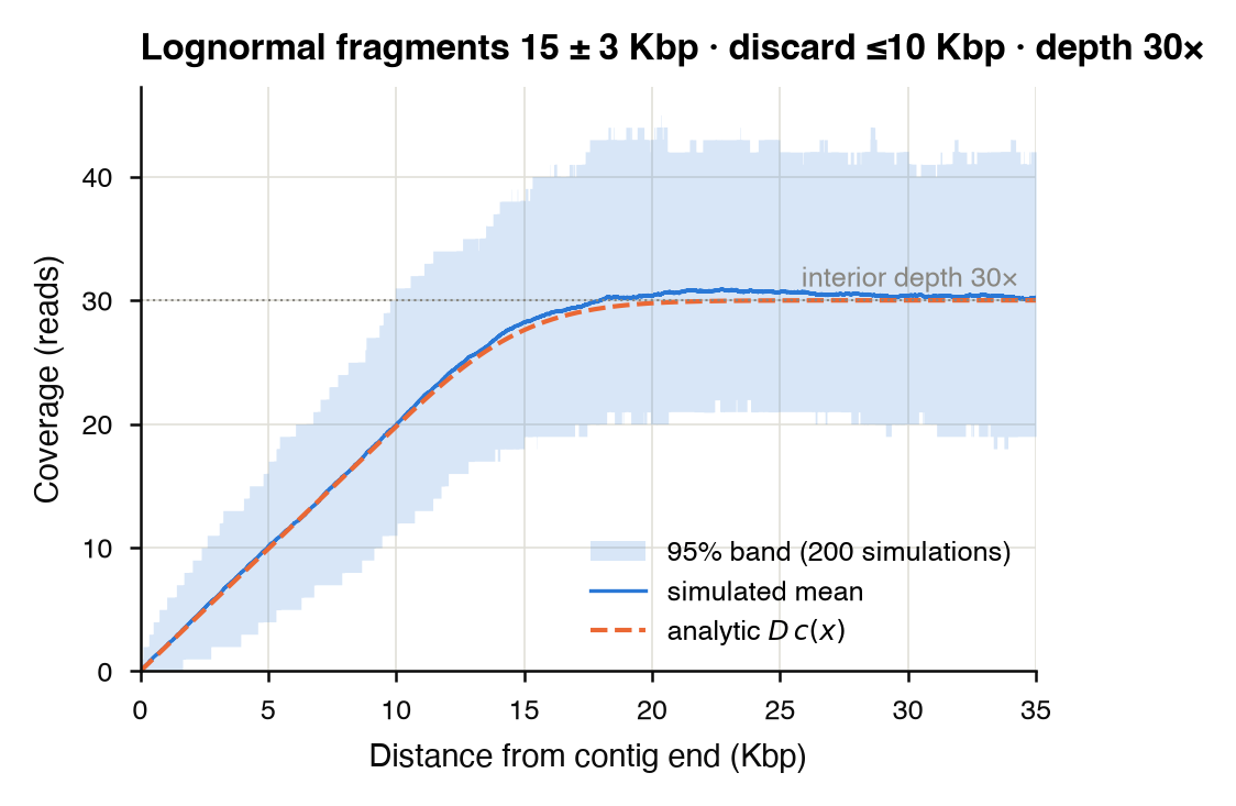
Simulation confirms the analytic curve. Each simulation fragments a 1 Mbp molecule with lognormal fragment lengths (mean 15 Kbp, sd 3 Kbp), discards fragments below the 10 Kbp lower-bound cutoff, places the survivors at 30× interior depth, and tallies terminal coverage; the band spans the central 95% of 200 independent runs:

Simulated terminal coverage for lognormal fragment lengths with mean 15 Kbp and standard deviation 3 Kbp under a strict 10 Kbp lower-bound size-selection cutoff at thirty-fold interior depth, with a 95 percent bootstrap band from 200 simulations, overlaid with the analytic expectation, which tracks the simulated mean closely across the whole decay region.

Reproducing these figures

Both figures are generated by scripts/generate_model_figures.py using teloclip.model (install with pip install 'teloclip[model]'). The analytic curve, the simulator and the bootstrap band are all available as library functions in teloclip.model.decay.

Explore the parameters¶

Use the sliders to see how depth, read-length profile and size-selection cutoff shape the decay. The curve is the analytic \(c(x)\) computed in your browser; the readout reports expected absolute coverage near the terminus.

What this means for teloclip¶

Overhang reads are the survivors of this decay. A read can only carry an overhang if it covers the outermost base, where coverage is at its minimum — at 30× interior depth with the 15 ± 3 Kbp HiFi profile and a 10 Kbp cutoff, expect only a handful of reads to span any given terminus. Zero overhangs at one contig end is often just sampling, not a structural problem.
Depth for telomere recovery is set by \(D \cdot c(0^+)\), not \(D\). If you want, say, ≥5 candidate overhang reads per end, work back from the curve: interior depth must be several times higher than a naive estimate.
Be gentle with length filters. Mapping-time read-length cutoffs act exactly like library size selection in this model: every kilobase you add to the minimum read length pushes the depleted zone deeper and removes potential overhang evidence. Filter on alignment quality and anchor length (see how overhangs are defined) rather than raw length where you can.
Interpret the report's depth panels with the curve in mind. The extend report plots overhang depth per contig end; ends with few overhangs but healthy flanking coverage are consistent with this model, while ends where coverage collapses faster than the curve predicts may indicate misassembly or collapsed repeats.